Before we can start with neural networks, we should talk a bit more about Logistic Regression – without understanding Logistic Regression, we can not understand neural networks. Moreover, I have learned how to use math in WordPress so I need to try it.

As we already know, Logistic Regression tries to find linear hyperplane that separates two classes. Hyperplane is a thing that has one dimension less than the thing it is in. If we have 1-dimensional space (line), hyperplane is a one-dimensional point. If we have 3D space a hyperplane is a 2D plane. And if we have 784-dimensional space a hyperplane is a 783-dimensional space.

Let’s start with 1D example. We have a line and we want to separate it to two segments. We need to find or define one point that separates those two segments. We can define it like this . If , we get positive value from the equation and the point is in one segment (class). If , the result is negative and the sample is in the other class. In 3D it’s similar, we just need more parameters: . When we plug-in our sample, we can again decide if the equation returns positive or negative value. Easy

Generic definition of a hyperplane in n-dimensional space looks like this . If we use vectors and , we can define hyperplane using vector multiplication . But how to get those parameters (a.k.a weights) ? We need to learn them form training samples.

First of all, we will define labels as follows. if it’s a positive example and if it’s a negative one. We will only deal with two classes and cover multiple classes later. In our letter classification we will set if the training example is an ‘A’. Now we need to be able to somehow compare output from and . The trouble is that is an unbounded real number and we need to somehow make it comparable to which is zero or one. That’s where we will use logistic function (hence the name Logistic Regression). The details are described here, for us dummies it suffices to say that Logistic Function maps real numbers to interval 0 to 1 in a way that is good. Like really good. It’s so good I will give it a name . So now we have which returns numbers between zero and one.

Thanks to logistic function we can now compare results of our model with the training labels. Imagine that we have already obtained parameters , we can measure how well the parameters classify our training set. We just have to somehow calculate the distance from prediction. In ML the distance is called cost function. With linear regression people use cross-entropy and again, I will not go into details here. We just need to know that it returns 0 if our model classifies the sample correctly and some really really high number if it classifies it incorrectly.

If we put it together, we can calculate for each pair and . If model makes correct prediction, the cost is zero, if it mis-predicts, the cost is high. We can even calculate a sum over all training examples: . If the sum is large, our model is bad and if the sum is 0 our model is the best. Function is function of parameters , we have made our training samples and labels part of the function definition. Now the only thing we need is to find such so the function is as small as possible.

And that’s how the model learns. We needed all those strange functions just to make this final function nice, having only one global minimum and other nice properties. While it’s possible to find the minimum analytically, for practical reasons it’s usually found by using something called gradient descent. I will not go to the details, it basically just generates random parameters , calculates and then it does small change to parameters so the next is a bit smaller. It then iterates until it reaches the minimum. That’s all we need to know for now.
Please note that we need all those strange functions mainly for learning. When classifying, I can still calculate and if it’s positive, it’s a letter ‘A’ and if it’s negative it’s some other letter. The advantage of applying the logistic function is that I can interpret the result as a probability.

What about multiple classes? We can use one-vs-all classifier. We can train a classifier that is able to separate A’s from the rest of the letters. Then B’s from the rest and so on. For our 10 letters we can apply the algorithm described above ten-times. Or we can use few tricks and learn all the letters in one pass.

The first trick is to change our labeling method. Before, we set y=1 if the letter in training set was an ‘A’. With multiple letters, we will use for ‘A’, for ‘B’, for ‘C’ etc. We also need to train different set of parameters (weights) for each letter. We can add all the weights into one matrix and calculate the result using matrix multiplication ( is 10-dimensional vector now as well). If we put weights for each letter to as a row, our matrix will have 10 rows (one for each letter) and 784 columns (one for each pixel). Our sample has 784 rows. If we multiply the two, we will get 10 numbers. We then element-wise add 10-numbers from and pick the largest one. That’s our prediction. For learning, we will use softmax function instead of logistic function, but the rest remains the same. At the end of the learning we will get 10×784 + 10 numbers that define 10 hyperplanes separating letters in 784-dimensional space.

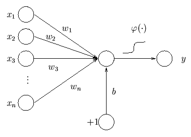
If case you are wondering why you need to know all of this, the reason is simple. Neural networks are built on top of ideas from logistic regression. In other words, logistic regression is one-layer neural network so in order to make real NN, we just need to add more layers. This is how our logistic regression looks like if depicted as a single neuron

Support Vector Machines, it sounds scary. Might be a name of some horror movie. Revenge of Support Vector Machines. But do not worry, for us dummies it’s not so complicated. I promise I will not use any intimidating words such as Lagrangian or Mercer’s Theorem. To make it even simpler, I will just talk about classification between two classes, as if we were trying to decide if a letter is an ‘A’ or not (please read previous post if you do not know what I am talking about).

SVMs are really similar to Logistic Regression, they try to find linear (hyper)plane that would separate our classes, one class on one side of the plane, the other on the other side. There are two important differences from Logistic Regression. The first one is that SVMs try to find plane that is as far as possible from both classes. But that’s not so interesting. When trying to classify letters, our problem is that most likely you can not find any such plane in our 784 dimensional space (28×28 pixels) that would separate A’s from other letters.

Imagine that we got to situation on the image below. For simplicity only in 2 dimension, as if our letters had only two pixels. (images taken from Everything You Wanted to Know about the Kernel Trick)

Imagine that our A’s are in the middle surrounded by their enemies, other letters. I just can not draw a straight line to separate them.

But I can escape to another dimension by creating a third feature like $latex x_1^2 + x_2^2$ (image on the right). Now I can separate the two classes. Look ma, I can draw a circle using a linear function!

While I can manually find a new feature that would separate the classes, I am to lazy to do that. It’s called Machine Learning, I want the machine to do it for me. SVMs can hep me with that. I can ask them to use a “kernel” which will make my model non-linear. Here is how it works, hopefully sufficiently dummified.

Imagine I have 20,000 training samples. The first thing the model does is that it remembers them all. It just shamelessly stores all 20k samples. Now imagine I have a new sample coming to the model. The model calculates distances from my 20k training samples to my new sample which results in 20k new features. First feature is the distance to the first sample in my training set, second is the distance to the second sample etc. Suddenly I have twenty-thousand-dimensional space and it’s much more likely that I will find a linear plane that would separate both classes. This method intuitively makes sense. Points representing A’s are likely to be near other point’s representing A’s so if we somehow incorporate distance into the model, it should get better result. In more clever sounding words, if I project the plane form 20k dimensional space back to my original 784 dimensional space, I can get highly nonlinear boundary.

Now a bit less dummified version (dummified is a word, I swear). Not all 20k training samples are used, only the most interesting ones (they are called Support Vectors hence the name). So the space we are using has less than 20k dimensions. Moreover the distance is not necessary a distance, it’s just some function that takes two points (vectors) as an input and returns a number (new feature). This function is called kernel and we pick it when configuring the classifier – Gaussian (rbf) is the most common. And while the method sounds complicated and slow, it uses some mathematical shortcuts so it’s relatively fast. Unfortunately it does not scale well with number of training samples.

Let’s see how the method looks in the code.

clf = svm.SVC(C=10, gamma=0.01, cache_size=2000) 

The rest of the code is the same as the last time, we’ve just changed the classifier. We see our favorite (hyper)parameter C. There is also a new parameter ‘gamma’ which configures the kernel. Smaller gamma makes our Support Vectors reach further and generalize more.

So what are the results? We got to 99.7% accuracy on the training set. It’s not surprising, the model actually remembers some of the training samples. If we call ‘clf.support_.shape’ it will tell us that it remembers 8,670 samples out of 20,000. It means that our model has to learn 8,670 parameters for each classified class. Let’s count how many numbers the model needs to remember. It stores 8,670 samples each of them having 28×28=784 values. We are trying to classify 10 letters so the model learns 10×8,670 parameters. (Actually 9×8,670, but let’s not go there.) All in all, the model consists of almost 7,000,000 parameters (numbers) most of it in form of Support Vectors picked from training samples. The training takes less than 3 minutes on my laptop.

What are the results on the validation set, on the samples that the model has not seen? It is 87%. The nonlinearity of the model gave us five more percent when compared to Logistic Regression. It’s great. The author of notMNIST set says that the set has ~6,5% label error rate so we need six more percent to get perfect. To confirm that I could not resist and run the classification on test set, which is much cleaner. I got 93% accuracy. Like 93% on this crazy images? Incredible. We still have further 6-7% to go and I am afraid we will have to resort to neural networks to get better results.

Sources:
Coursera Machine Learning Course
Everything You Wanted to Know about the Kernel Trick
scikit learn documentation on RBF SVM parameters
scikit learn documentation on SVC

Before we can move to more advanced topics, we should discuss over and underfitting. It reminded me my high school biology lessons. We were expected to recognize different kinds of flowers. In the lessons we were given images of flowers and we were supposed to learn that this flower is yellow and has this type of leafs and this one is blue with different kind of leafs. But there was an alternative strategy how to pass the exam. The images had numbers in the corner and it’s been much more easier to memorize the numbers with corresponding names. You did not learn anything about the flowers but if your only objective was to pass the exam, it was perfect.

And exactly the same problem we have in machine learning. If you do not have many training examples and you have complicated model, the learning algorithm may just memorize the training samples without trying to generalize. It basically does the same thing what my classmates did in the biology lessons. It is great if you only want to classify samples from the training set. If you however want to classify unknown samples, you want your algorithm to generalize.

Let’s look at some examples. I will use the same algorithm as the last time on notMNIST data, I will just make the training set smaller, let’s say 1k samples. In noMNIST set there are 10 letters A-J. We have shuffled our training set so in those 1k samples there will be around 100 samples of each letter. I am using Logistic Regression in 784 dimensional space which maps to those 10 classes. We also have bias elements for each class so the model has 7850 parameters. Parameters are just some numbers which the algorithm learns based on the samples. We dummies do not need to know more. So the algorithm learns ~8000 numbers from 1000 samples. Or for each letter ~800 parameters from ~100 samples. There is quite substantial danger that the model will just memorize the training set.

from sklearn import linear_model

clf_l = linear_model.LogisticRegression()
# we do not want to use the whole set
size = 1000

# images are 28x28, we have to make a vector from them
tr = train_dataset[:size,:,:].reshape(size, 784)

# This is the most important line. I just feed the model training samples and it learns
clf_l.fit(tr, train_labels[:size])

# This is prediction on training set
prd_tr = clf_l.predict(tr)
print(float(sum(prd_tr == train_labels[:size]))/prd_tr.shape[0])

# let's check if the model is not cheating, it has never seen this letters before
prd_l = clf_l.predict(valid_dataset.reshape(valid_dataset.shape[0], 784))
float(sum(prd_l == valid_labels))/prd_l.shape[0]

And indeed, the model has been able to correctly classify 99% of the samples from the training set. That’s why we have the validation set. We will use it to check our model. It’s as if our biology teacher had one set of images for the lessons and another set for the exams. Actually, it’s more complicated, we have also test set, but we will not be using that one so often so let’s forget about it for now.

Our model is able to recognize 74% of samples from our validation set. Not to bad. Luckily for us, Logistic Regression is just trying to find linear (flat) plane to split the space so it is not able to cheat much. It can not simply pick the training examples, it has to take half of the space with them. But let’s try to force it to cheat anyway. Logistic Regression has parameter C (as for cheating) which says how much we allow the algorithm to over-fit. Higher C means more cheating, lower C means less cheating (for those who are used to more usual notation C = 1/lambda)

# Cheating level Carnage
clf_l = linear_model.LogisticRegression(C=100)

If we tune cheating parameter to 100, we get 99.9% of success on training set and 71% on validation set. If we use a value from other side of the spectrum C=0.001 we get 75% on training set and 76% on validation set. It’s up to us to decide what is better. Here is a table for some values of C for 1k samples.

Another other way for preventing overfitting is to provide more training examples. Imagine our biology lesson with much more samples with different numbers. From certain number of samples, it is much easier to try to learn how to recognize those damn flowers than to try to memorize all the numbers in the corner. And the same applies for machine learning algorithms too. If I use C=100 with 10k training samples, I get 93% accuracy on training set and 74% on validation set. You can notice that it’s actually worse than most of the results with 1k of examples and different C values. But we can combine both approaches. Let’s say that I pick C=0.01 and use 20k training samples. I get 83% accuracy on training set and 82% on validation set. As you can see, both numbers are converging. There is only 1% difference. It means that we are approaching limits of our model. Using more samples is not likely to help much. I am afraid we have to move to better model to get better results. That’s it for today. You can go now.

Update: Fixed number of parameters