Last time we have discussed word2vec algorithm, today I’d like to show you some of the results.

They are fascinating. Please remember that word2vec is an unsupervised algorithm, you just feed it a lot of text and it learns itself. You do not have to tell it anything about the language, grammar, rules, it just learns by reading.

What’s more, people from Google have published a model that is already trained on Google news, so you can just download the model, load it to you Python interpreter and play. The model has about 3.4G and contains 3M words, each of them represented as a 300-dimensional vector. Here is the source I have used for my experiments.

from gensim.models import Word2Vec
model = Word2Vec.load_word2vec_format('GoogleNews-vectors-negative300.bin', binary=True)
# take father, subtract man and add woman
model.most_similar(positive=['father', 'woman'], negative=['man'])

[('mother', 0.8462507128715515),
 ('daughter', 0.7899606227874756),
 ('husband', 0.7560455799102783),
 ('son', 0.7279756665229797),
 ('eldest_daughter', 0.7120418548583984),
 ('niece', 0.7096832990646362),
 ('aunt', 0.6960804462432861),
 ('grandmother', 0.6897341012954712),
 ('sister', 0.6895190477371216),
 ('daughters', 0.6731119751930237)]

You see, you can take vector for “father” subtract “man” and add “woman” and you will get “mother”. Cool. How does it work? As we have discussed the last time, word2vec groups similar words together and luckily it also somehow discovers relations between the words. While it’s hard to visualize the relations in 300-dimensional space, we can project the vectors to 2D.

plot("man woman father mother daughter son grandmother grandfather".split())

Now you see how it works, if you want to move from “father“ to “mother“, you just move down by the distance which is between “man” and “woman”. You can see that the model is not perfect. One would expect the distance between “mother” and “daughter” will be the same as between “father” and “son”. Here it is much shorter. Actually, maybe it corresponds to reality.

Let’s try something more complicated

plot("pizza hamburger car motorcycle lamb lamp cat cow sushi horse pork pig".split())

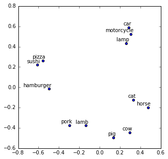
In this example, we loose lot of information by projecting it to 2D, but we can see the structure anyway. We have food on the left, meat in the middle, animals on the right and inanimate objects at the top. Lamb and lamp sound similar but it did not confuse the model. It just is not sure if a lamb it’s meat or an animal.

And now on something completely different – names.

plot("Joseph David Michael Jane Olivia Emma Ava Bill Alex Chris Max Theo".split())

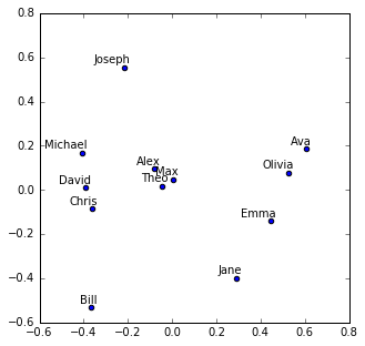
Guys on the left, gals on the right and unisex in the middle. I wonder, though what the vertical axis means.

I have played with the model for hours and it does not cease to surprise me. It just reads the text and learns so much, incredible. If you do not want to play with my code you can also try it online.

Last time we have skimmed through neural networks. Today I’d like to describe one cool algorithm that is based on them.

Up until now we have worked on character recognition in images. It’s quite straightforward to convert an image to numbers, we just take pixel intensities and we have numbers. But what to do if we want to work with text? We can not do matrix multiplication with words, we need to somehow convert them to numbers. One way to do it is just take all words and number them. ‘aardvark’ would be 1, ‘aardwolf’ 2 etc. The problem with this approach is that similar words would have completely different numbers. Let’s say you are working on image recognition. You want to have a model that says “This is most likely a cat, but maybe it’s a kitten or a tiger. It definitely is something cat-like”. For this it’s better to have numeric representations of cat, kitten and tiger that are similar. Since we are dummies, I will not try to find mathematical reasons for this. Intuition tells me that pictures of kitten and cat are quite similar so it makes sense that output of the learning algorithm should be similar as well. It’s much harder to teach it if cat has number 10 and kitten 123,564.

But how to get such representations? We can use word2vec which allows us to map words to a n-dimensional vector space in a way that puts similar words together. The trick is quite simple. Similar words are used in similar contexts. I can say “I like pizza with cheese”. Or “I like hamburger with cheese”. Here the contexts are similar, just the food is different. Now I just need some algorithm that would read lot of text and somehow find words that are used in similar contexts and put them together.

Word2vec takes a neural network and teaches it to guess contexts based on words. As an input I can take a word “pizza” and try to teach the network to come up with “I like … with cheese”. This approach is called skip-gram. Or I can try the other direction and teach the network to answer “pizza” if I feed it “I like … with cheese.” This direction is called CBOW. There are some differences in the results, but thay are not important enough for now. In the next text I will describe skip-gram with 4 words in the context.

Let’s take a look at the details. We will take simple neural network with one hidden layer. On the input, I will use one-hot encoding. ‘aardvark’ would be [1,0,0,…], ‘aardwolf’ [0,1,0,…], each word would be represented by a vector with zeros and one ‘1’. If my dictionary has 50k words I would end up with 50k-dimensional input vector. We have the input, let’s move to the hidden layer. The size of the hidden layer is up to me, at the end it will be the size of the vector representing the word. Let’s pick 128. Then there will be an output layer that would map the data back to one-hot encoded vector of context words. The network will take large sparse vector, squeeze it into much smaller and denser one and then unsqueeze it to a large vector again.

I take “pizza”, convert it to a 50k-dimensional vector with only one nonzero value. Then I multiply this vector with 128x50k-dimensional matrix and I get 128-dimensional vector. I take this vector, multiply it with another 50k x128-dimensional matrix and get 50k dimensional vector. After the right normalization, this vector will contain probability that given word occurs in context of word “pizza”. Value on the first position will be quite low, aardvark and pizza are not usually used in the same sentence. Actually, I just did that, so the next time this text gets to a learning algorithm, the first value in the vector will be slightly larger.

Of course I have to somehow get those matrices, but it’s just neural network training with some dirty tricks to make it computable. The trouble is, that the dictionary can by larger than 50k words so the learning phase is not trivial. But I am a dummy, I do not care. I just need to know that I will feed it the whole internet (minus porn) and it will somehow learn to predict the context.

Ok, we have a neural network that can predict the context, where do I get the vectors representing the words? They are in the first matrix from the model. That’s the beauty of it. Imagine that I have “pizza” on the input. It’s a vector with all zeros and one “1”. The matrix multiplication is not a multiplication at all, it just picks one column of the first matrix in the model. One column is just 128-dimensional vector and when we multiply it with the second matrix we want to get probabilities that given word is in the context. I guess that “like”, “eat”, “dinner”, “cheese” or “bacon” will be quite high. Now let’s feed in “hamburger”. It will pick another column from the first matrix, but we expect similar words in the result. Not the same, but similar. And to get similar results, we need similar vector in the hidden layer so when we multiply it with the second matrix we get similar context words. But the vector in hidden layer is just a column in the first matrix. It means, that in order to get similar results for words with similar contexts, the columns in the first matrix have to be similar (well they do not have to, but it usually ends up this way)

It’s quite beautiful and powerful algorithm. What’s more, the positions of the vectors in the vector space have some structure too. You have most likely seen the example where they take vector for “king” subtract vector for “man” and add vector for “women” and they get dangerously close to vector for “queen”. I have no idea why it works this way, but it does.

That’s all for today, next time I will try to show you some results. Here is some visualization you can admire in the meantime.

Sources:
Tensorflow tutorial
Nice (long) lecture about word2vec details
Visualization of High Dimensional Data using t-SNE with R
Just Google the rest

Even though Neural Networks are the most cool thing in machine learning, they conceptually are just multiple linear regressions chained one after the other. So I will not draw any fancy pictures of neurons, I will just write boring matrix multiplications. Both representations are equivalent.

Last time, we have learned that logistic regression classification is just matter taking sample , multiplying it by matrix and adding some constant bias term . In our letter recognition example is 784-dimensional vector, is 10×784 dimensional matrix and is 10-dimensional vector. Once our model learns weights and , we just calculate and pick the row with the maximal value. Index of the row is our class prediction.

The downside of logistic regression is that it can only classify classes that are separable by linear plane. We can fix that by adding multiple linear regressions one after each other.

Let’s say that we take the input, multiply it by a matrix, add bias and then take the output. We can again multiply it by another matrix and add another bias We then can take the result of this second operation and use it as our prediction.

We will call this Neural Network with one hidden layer. The hidden layer is the vector . It is hidden because nobody sees it, it’s just something internal to the model. It’s up to us to decide what the size of will be. The size is usually called number of neurons in the hidden layer. We can even add more hidden layers, each with different size. Unfortunately no one will tell you how many layers and how big they should be, you have to play with the parameters and see how the network performs.

To make things even more complicated, you can also use activation function. Activation function can take the result of each layer and make it more non-linear. So we will get where is the activation function. Popular choices are relu, tanh and for the last layer softmax.

Luckily for us, it’s quite simple to play with neural networks in Python. There are several libraries, I have picked Keras, since it’s quite powerful and easy to use.

from keras.models import Sequential
from keras.layers.core import Dense, Activation
from keras.optimizers import SGD

model = Sequential()
# Hidden layer with 1024 neurons
model.add(Dense(output_dim=1024, input_dim=image_size * image_size, init="glorot_uniform"))
# ReLU activation
model.add(Activation("relu"))
# We have 10 letters
model.add(Dense(output_dim=10, init="glorot_uniform"))
# Softmax makes sense for the activation of the output layer
model.add(Activation("softmax"))

# Let the magic happen
model.compile(loss='categorical_crossentropy', optimizer=SGD())

model.fit(train_dataset, train_labels, batch_size=128, nb_epoch=50)

In this example we will create a neural network with one hidden layer of 1024 neurons with activation function ReLU. In other words (ignoring biases), we will take the pixels of the letter, multiply them by a matrix which will result in 1024 numbers. We will then set all the negative numbers to 0 (ReLU) and then multiply the result by another matrix to get 10 numbers. We then find the highest of those numbers. Let’s say that highest result is in second row then the resulting letter is B.

We of course need to train the network. It’s more complex, luckily we do not need to know much about it. So let’s just use Stochastic Gradient Descent with batch size 128. nb_epoch says that we should walk through all training examples 50-times. Please remember that training is just finding of the minimum of some loss function.

I am using Keras with Tensorflow so when I call model.compile it actually generates some optimized distributed parallel C++ code that can even run on GPU. The code will train the network for us. This is important, large networks with lots of hidden layers and lots of parameters can take ages and lot of calculations to learn. Keras and Tensorflow hides the complexity so I do not have to worry about it.

And what about the results? We get 96% accuracy on test set! Another 3% increase from SVM. Since the best result on notMNIS is allegedly 97.1% I think it’s not bad at all. Can you calculate how many parameters we do have? In the first layer we have matrix of 1024×784 parameters + 1024 bias terms. In the output layer we have 10×1024 + 10 parameters. In total it’s around 800,000 parameters. Training takes around 20 minutes on my laptop.