Category Archives: Articles in English

Machine Learning for dummies – overfitting

Before we can move to more advanced topics, we should discuss over and underfitting. It reminded me my high school biology lessons. We were expected to recognize different kinds of flowers. In the lessons we were given images of flowers and we were supposed to learn that this flower is yellow and has this type of leafs and this one is blue with different kind of leafs. But there was an alternative strategy how to pass the exam. The images had numbers in the corner and it’s been much more easier to memorize the numbers with corresponding names. You did not learn anything about the flowers but if your only objective was to pass the exam, it was perfect.

And exactly the same problem we have in machine learning. If you do not have many training examples and you have complicated model, the learning algorithm may just memorize the training samples without trying to generalize. It basically does the same thing what my classmates did in the biology lessons. It is great if you only want to classify samples from the training set. If you however want to classify unknown samples, you want your algorithm to generalize.

Let’s look at some examples. I will use the same algorithm as the last time on notMNIST data, I will just make the training set smaller, let’s say 1k samples. In noMNIST set there are 10 letters A-J. We have shuffled our training set so in those 1k samples there will be around 100 samples of each letter. I am using Logistic Regression in 784 dimensional space which maps to those 10 classes. We also have bias elements for each class so the model has 7850 parameters. Parameters are just some numbers which the algorithm learns based on the samples. We dummies do not need to know more. So the algorithm learns ~8000 numbers from 1000 samples. Or for each letter ~800 parameters from ~100 samples. There is quite substantial danger that the model will just memorize the training set.

from sklearn import linear_model

clf_l = linear_model.LogisticRegression()
# we do not want to use the whole set
size = 1000

# images are 28x28, we have to make a vector from them
tr = train_dataset[:size,:,:].reshape(size, 784)

# This is the most important line. I just feed the model training samples and it learns
clf_l.fit(tr, train_labels[:size])

# This is prediction on training set
prd_tr = clf_l.predict(tr)
print(float(sum(prd_tr == train_labels[:size]))/prd_tr.shape[0])

# let's check if the model is not cheating, it has never seen this letters before
prd_l = clf_l.predict(valid_dataset.reshape(valid_dataset.shape[0], 784))
float(sum(prd_l == valid_labels))/prd_l.shape[0]

And indeed, the model has been able to correctly classify 99% of the samples from the training set. That’s why we have the validation set. We will use it to check our model. It’s as if our biology teacher had one set of images for the lessons and another set for the exams. Actually, it’s more complicated, we have also test set, but we will not be using that one so often so let’s forget about it for now.

Our model is able to recognize 74% of samples from our validation set. Not to bad. Luckily for us, Logistic Regression is just trying to find linear (flat) plane to split the space so it is not able to cheat much. It can not simply pick the training examples, it has to take half of the space with them. But let’s try to force it to cheat anyway. Logistic Regression has parameter C (as for cheating) which says how much we allow the algorithm to over-fit. Higher C means more cheating, lower C means less cheating (for those who are used to more usual notation C = 1/lambda)

# Cheating level Carnage
clf_l = linear_model.LogisticRegression(C=100)

If we tune cheating parameter to 100, we get 99.9% of success on training set and 71% on validation set. If we use a value from other side of the spectrum C=0.001 we get 75% on training set and 76% on validation set. It’s up to us to decide what is better. Here is a table for some values of C for 1k samples.

C tr. set valid. set
0.001 75% 76%
0.01 81% 79%
0.1 92% 78%
1 99% 75%
10 99% 72%
100 99.9% 71%

Another other way for preventing overfitting is to provide more training examples. Imagine our biology lesson with much more samples with different numbers. From certain number of samples, it is much easier to try to learn how to recognize those damn flowers than to try to memorize all the numbers in the corner. And the same applies for machine learning algorithms too. If I use C=100 with 10k training samples, I get 93% accuracy on training set and 74% on validation set. You can notice that it’s actually worse than most of the results with 1k of examples and different C values. But we can combine both approaches. Let’s say that I pick C=0.01 and use 20k training samples. I get 83% accuracy on training set and 82% on validation set. As you can see, both numbers are converging. There is only 1% difference. It means that we are approaching limits of our model. Using more samples is not likely to help much. I am afraid we have to move to better model to get better results. That’s it for today. You can go now.

Update: Fixed number of parameters
Machine learning for dummies – Logistic Regression

Hi, welcome to my on-line course “machine learning for dummies”. Usually courses like this are written by an expert. This is not my case, though. I do not know anything about machine learning. I have spent more than 10 years working with server side Java, moving data here and there. I have even worked as REST API architect or Scrum master. Yes, the Scrum that eats programmers soul. But no machine learning whatsoever apart from image recognition course at the university 12 years ago and Machine Learning course on Coursera few months ago. But now I have decided that I will learn ML, so I quit my job, declined an interesting offer and started to learn ML.

Since Deep learning is the current hype, I have started with Deep Learning course at Udacity. Deep learning course from Google right in my living room? Cool.

And the course went quite well until the very first exercise which was about recognizing notMnist dataset

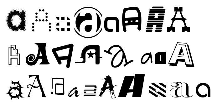
notMNIST

You have this “letters” and you want to recognize them. Sounds like a job for machine learning, right?

Installing Python libraries

To finish the exercise, you need to know something about machine learning and Python first. I do not know neither. Python is quite simple, if you know programming you will learn it in no time. The most complex task is the installation. I have spent like six hours trying to install all the required libraries. If you do not know Python, you just have no idea if you want to use OS specific packages (apt, brew), pip, easy_install or whatnot. The thing is, in Java you have projects that describe their dependencies using Maven or Gradle. So if you want to work on Java project, you just execute ‘mvn test’, it downloads half of the Internet and you are done. But in Python you have no project so you have to download all libraries yourself. What’s more, those libraries depend on each other and you need to have correct versions. Well I downloaded and recompiled half of the Internet multiple times, every time getting different conflict (most often between matplotlib and numpy). Luckily, people using Python know that their package systems suck so they provide Docker images with all the libraries installed. I have used the image to figure out which version of libraries work together. Today, I was trying to install it again on Mac OS and I was able to do it under an hour using Anaconda so maybe this Python distribution system works better than the others.

But once you have Python with all the libraries installed, you get your superpowers. Thanks to numpy, you can easily work with matrices, thanks to matplotlib you can plot charts and thanks to scikit-learn you can do machine learning without knowing much about it. That’s what I need.

Logistic Regression

So back to our notMnist example. After I have reviewed most of the Coursera course I have learned that in machine learning you need features – the data you will use in your algorithm. But we have images, not features. The most naive approach is to take the pixels and use them as features. Images in notMNIST are 28×28 pixel, so for each image we have 784 numbers (shades of gray). We can create 784 dimensional space and represent each image as one point in this space. Please think about it for a while. I will create really high dimensional space and represent each sample (image) by one point in the space. The idea is that if I have the right set of features, the points in this space will became separable. In other words, I will be able to split the space into two parts, one that contains points representing letters A and another part with all other letters. This is called Logistic Regression and there are implementation that do exactly that. Basically you just need to feed the algorithm samples with correct labels and it tries to figure out how to separate those points in the high-dimensional space. Once the algorithm finds the (hyper)plane that separates ‘A’s from other letters, you have your classifier. For each new letter you just check in which part of the space the corresponding point is and you know if it’s an A or not. Piece of cake.

But if you think about it, it just can not work. You just feed it raw pixels. Look at the images above, you are trying to recognize letter ‘A’ just based on values of the pixels. But each of the ‘A’s above is completely different. The learning algorithm just can not learn to recognize the letter just based on individual pixels. Or can it?

What’s more, I am trying to find a flat plane that would separate all As in my 784 dimensional space from all other letters. What if As in my crazy space form a little island which is surrounded by other letters. I just can not separate them by a flat plane. Or can I?

Well surprisingly I can and it is quite easy to implement

from sklearn import linear_model

clf_l = linear_model.LogisticRegression()
# we do not want to use the whole set, my old CPU would just melt
size = 20000 

# images are 28x28, we have to make a vector from them
tr = train_dataset[:size,:,:].reshape(size, 784)

# This is the most important line. I just feed the model 20k examples and it learns
clf_l.fit(tr, train_labels[:size])

# This is prediction on training set
prd_tr = clf_l.predict(tr)
print(float(sum(prd_tr == train_labels[:size]))/prd_tr.shape[0])
# prints 0.86 we are able to recognize 86% of the letters in the training set

# let's check if the model is not cheating, it has never seen
# the letters from the validation set before
prd_l = clf_l.predict(valid_dataset.reshape(valid_dataset.shape[0], 784))
float(sum(prd_l == valid_labels))/prd_l.shape[0]
# Cool 80% matches

Even this method that just can’t work is able to classify 80% of letters it has never seen before.

You can even easily visualize the letters that did not match

import numpy
import matplotlib.cm as cm

def num2char(num):
    return chr(num + ord('a'))

# indexes of letters that do not match 
# change the last number to get another letter
idx = numpy.where(prd_l != valid_labels)[0][17]
print("Model predicts: " + num2char(clf_l.predict(valid_dataset[idx].reshape(1, 784))))
print("Should be: " +num2char(valid_labels[idx]))
%matplotlib inline
plt.imshow(valid_dataset[idx,:,:] + 128,cmap = cm.Greys_r)

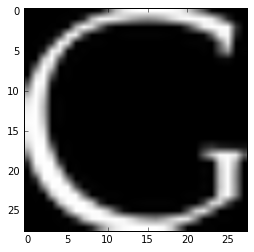
G

This should have been G but the model has classified it as C. Understandable mistake. Another letter is even better.

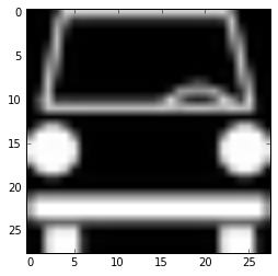
f

This obvious ‘f’ has been incorrectly classified as A. Well, to me it looks more like an A than an f. The thing is that even this simple naive model mostly does “understandable” mistakes only. Either the misclassified letter is not a letter at all or the classifier makes mistake because the letters are really similar. Like I and J, I and F and so on.

So what we have learned today? First of all that even stupid model on stupid features can work surprisingly well. Secondly that Python libraries are not easy to install but easy to use. Here I have to admit that similar code in Java would have been just crazy.

Next time we will try SVM and maybe try to figure out some better features to make our model even better.

Converting RxJava Observables to Java 8 Completable future and back

I have been working on a small project that converts between different types of Java futures. The most challenging conversion is from/to RxJava observable. The reason is simple – RxJava observable is quite different than let’s say Java 8 CompletableFuture. Observable can produce multiple values, future can handle at most one, observable revolves around non-blocking push paradigm, futures mix blocking and non-blocking approach into one API. Nevertheless, the conversion is quite straightforward.

Let’s say that we want to create a CompletableFuture that handles first item of an bservable. It’s quite simple.

public class ObservableCompletableFuture<T> extends CompletableFuture<T> {
    private final Subscription subscription;
    public ObservableCompletableFuture(Observable<T> observable) {
        subscription = observable.single().subscribe(
                this::complete,
                this::completeExceptionally
        );
    }

    @Override
    public boolean cancel(boolean mayInterruptIfRunning) {
        subscription.unsubscribe();
        return super.cancel(mayInterruptIfRunning);
    }
}

We extend CompletableFuture and then we just subscribe to the observable. Subscribe method accepts two actions. The first will be called when an item is produced, the other one upon error. By calling single() method on Observable we make sure that at most one item will be produced.

The only thing missing is to unsubscribe upon cancel.

What about the opposite direction, if we want to convert CompletableFuture to Observable? It’s simple as well.

public class CompletableFutureObservable<T> extends Observable<T> {
    CompletableFutureObservable(CompletableFuture<T> completableFuture) {
        super(onSubscribe(completableFuture));
    }

    private static <T> OnSubscribe<T> onSubscribe(final CompletableFuture<T> completableFuture) {
        return subscriber -> {
            completableFuture.thenAccept(value -> {
                if (!subscriber.isUnsubscribed()) {
                    subscriber.onNext(value);
                    subscriber.onCompleted();
                }
                }).exceptionally(throwable -> {
                if (!subscriber.isUnsubscribed()) {
                    subscriber.onError(throwable);
                }
                return null;
            });
        };
    }
}

We just have to describe what to do if someone subscribes to the observable. We just register two callbacks on the CompletableFuture. The first one using thenAccept calls onNext and onCompleted when the CompletableFuture value is ready. The other one calls onError in case of error. Please note that we do not cancel the future if the subscriber unsubscribes. We can not do it, since we do not know how many subscriptions are registered. And even if we knew, we do not know how the future will be used.

Apart from that, the implementation is pretty straightforward. Please note how helpful the lambdas and method references are, without them the code would be much more verbose. If you are interested in the details, do not hesitate to check the code.